In Chapter 4.
parameterization of ![]() have been studied.
This section now discusses parameterizations
of the prior density
have been studied.
This section now discusses parameterizations
of the prior density ![]() .
For Gaussian prior densities
that means parameterization of mean and/or covariance.
The parameters of the prior functional,
which we will denote by
.
For Gaussian prior densities
that means parameterization of mean and/or covariance.
The parameters of the prior functional,
which we will denote by ![]() ,
are in a Bayesian context also known as hyperparameters.
Hyperparameters
,
are in a Bayesian context also known as hyperparameters.
Hyperparameters ![]() can be considered
as part of the hidden variables.
can be considered
as part of the hidden variables.
In a full Bayesian approach the ![]() -integral
therefore has to be completed
by an integral over the additional hidden variables
-integral
therefore has to be completed
by an integral over the additional hidden variables ![]() .
Analogously, the prior densities
can be supplemented by priors for
.
Analogously, the prior densities
can be supplemented by priors for ![]() ,
also be called hyperpriors,
with corresponding energies
,
also be called hyperpriors,
with corresponding energies ![]() .
.
In saddle point approximation
thus an additional stationarity equation
will appear,
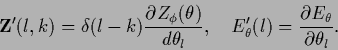
resulting from the derivative
with respect to ![]() .
The saddle point approximation of the
.
The saddle point approximation of the ![]() -integration
(in the case of uniform hyperprior
-integration
(in the case of uniform hyperprior ![]() and with the
and with the ![]() -integral being calculated exactly or by approximation)
is also known as ML-II prior [16]
or evidence framework
[85,86,213,147,148,149,24].
-integral being calculated exactly or by approximation)
is also known as ML-II prior [16]
or evidence framework
[85,86,213,147,148,149,24].
There are some cases where it is convenient
to let the likelihood ![]() depend, besides on a function
depend, besides on a function ![]() ,
on a few additional parameters.
In regression such a parameter
can be the variance of the likelihood.
Another example is the inverse temperature
,
on a few additional parameters.
In regression such a parameter
can be the variance of the likelihood.
Another example is the inverse temperature ![]() introduced in
Section 6.3,
which, like
introduced in
Section 6.3,
which, like ![]() also appears in the prior.
Such parameters may formally be added to
the ``direct'' hidden variables
also appears in the prior.
Such parameters may formally be added to
the ``direct'' hidden variables
![]() yielding an enlarged
yielding an enlarged ![]() .
As those ``additional likelihood parameters''
are like other hyperparameters typically
just real numbers, and not functions like
.
As those ``additional likelihood parameters''
are like other hyperparameters typically
just real numbers, and not functions like ![]() ,
they can often be treated analogously to hyperparameters.
For example, they may also be determined by cross-validation (see below)
or by a low dimensional integration.
In contrast to pure prior parameters, however,
the functional derivatives with respect to such
``additional likelihood parameters''
contain terms arising from the derivative of the likelihood.
,
they can often be treated analogously to hyperparameters.
For example, they may also be determined by cross-validation (see below)
or by a low dimensional integration.
In contrast to pure prior parameters, however,
the functional derivatives with respect to such
``additional likelihood parameters''
contain terms arising from the derivative of the likelihood.
Within the Frequentist interpretation of error minimization
as empirical risk minimization
hyperparameters ![]() can be determined by
minimizing the empirical generalization error
on a new set of test or validation data
can be determined by
minimizing the empirical generalization error
on a new set of test or validation data ![]() being independent from the training data
being independent from the training data ![]() .
Here the empirical generalization error is meant to be
the pure data term
.
Here the empirical generalization error is meant to be
the pure data term
![]() =
=
![]() of the error functional
for
of the error functional
for ![]() being the optimal
being the optimal ![]() for the full regularized
for the full regularized
![]() at
at ![]() and for given training data
and for given training data ![]() .
Elaborated techniques include
cross-validation and bootstrap methods
which have been mentioned in Sections 2.5
and 4.9.
.
Elaborated techniques include
cross-validation and bootstrap methods
which have been mentioned in Sections 2.5
and 4.9.
Within the Bayesian interpretation
of error minimization as posterior maximization
the introduction of hyperparameters
leads to a new difficulty.
The problem arises from the fact
that it is usually desirable
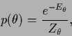
to interpret the error term ![]() as prior energy for
as prior energy for ![]() , meaning that
, meaning that
| (420) |
| (421) |
 |
(422) |
| (423) |
| (424) |
It is interesting to look what happens
if
![]() of Eq. (419)
is expressed
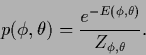
in terms of joint energy
of Eq. (419)
is expressed
in terms of joint energy
![]() as follows
as follows
 |
(425) |
| (426) |
Notice especially,
that this discussion also applies to the case
where ![]() is assumed to be uniform
so it does not have to appear explicitly in the error functional.
The two ways of expressing
is assumed to be uniform
so it does not have to appear explicitly in the error functional.
The two ways of expressing
![]() by a joint or conditional energy, respectively,
are equivalent
if the joint density factorizes.
In that case, however,
by a joint or conditional energy, respectively,
are equivalent
if the joint density factorizes.
In that case, however,
![]() and
and ![]() are independent,
so
are independent,
so ![]() cannot be used to parameterize the density of
cannot be used to parameterize the density of ![]() .
.
Numerically the need to calculate
![]() can be disastrous
because normalization factors
can be disastrous
because normalization factors
![]() represent often an extremely high dimensional (functional) integral
and are, in contrast to the normalization of
represent often an extremely high dimensional (functional) integral
and are, in contrast to the normalization of ![]() over
over ![]() ,
very difficult to calculate.
,
very difficult to calculate.
There are, however,
situations for which
![]() remains
remains ![]() -independent.
Let
-independent.
Let
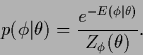
![]() stand for example
for a Gaussian specific prior
stand for example
for a Gaussian specific prior
![]() (with the normalization condition factored out
as in Eq. (90)).
Then, because the normalization of a Gaussian is independent
of its mean, parameterizing the mean
(with the normalization condition factored out
as in Eq. (90)).
Then, because the normalization of a Gaussian is independent
of its mean, parameterizing the mean ![]() =
= ![]() results in
a
results in
a ![]() -independent
-independent
![]() .
.
Besides their mean, Gaussian processes are
characterized by their covariance operators
![]() .
Because the normalization only depends on
.
Because the normalization only depends on
![]() a second possibility
yielding
a second possibility
yielding ![]() -dependent
-dependent
![]() are parameterized transformations of the form
are parameterized transformations of the form
![]() with orthogonal
with orthogonal ![]() =
=
![]() .
Indeed, such transformations do not change the determinant
.
Indeed, such transformations do not change the determinant
![]() .
They are only non-trivial for multi-dimensional Gaussians.
.
They are only non-trivial for multi-dimensional Gaussians.
For general parameterizations of density estimation problems, however,
the normalization term
![]() must be included.
The only way to get rid of that normalization term
would be to assume a compensating hyperprior
must be included.
The only way to get rid of that normalization term
would be to assume a compensating hyperprior
| (427) |
Thus, in the general case we have to consider the functional
 |
(431) |
Finally, we want to remark that
in case function evaluation of
![]() is much cheaper than calculating the gradient (430),
minimization methods not using the gradient
should be considered, like for example the
downhill simplex method
[196].
is much cheaper than calculating the gradient (430),
minimization methods not using the gradient
should be considered, like for example the
downhill simplex method
[196].