In this section we look at some numerical examples and discuss implementations of the nonparametric learning algorithms for density estimation we have discussed in this paper.
As example,
consider a problem
with a one-dimensional ![]() -space
and a one-dimensional
-space
and a one-dimensional ![]() -space,
and a smoothness prior
with inverse covariance
-space,
and a smoothness prior
with inverse covariance
| (706) | |||
| (707) |
| (708) |
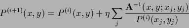
We will now study nonparametric density estimation
with prior factors being Gaussian with respect to ![]() as well as being Gaussian with respect to
as well as being Gaussian with respect to ![]() .
.
The error or energy functional for a Gaussian prior factor in ![]() is given by Eq. (108).
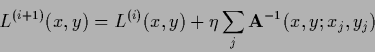
The corresponding iteration procedure is
is given by Eq. (108).
The corresponding iteration procedure is
 |
(710) |
![\begin{displaymath}
\left.
\!-\!
\left(
\sum_j \! \delta(x^\prime\! -\!x_j)
\!+...
...e\prime} )
\right)
\!e^{L^{(i)}(x^\prime ,y^\prime )}
\right].
\end{displaymath}](img2352.png)
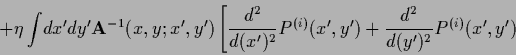
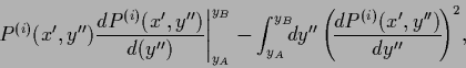
Analogously,
for error functional ![]() (164) the iteration procedure
(164) the iteration procedure
| (711) |
 |
(712) |
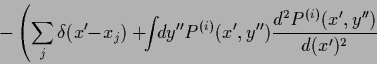
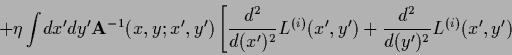
![\begin{displaymath}
\left.\left.
+\int \!dy^{\prime\prime} P^{(i)} (x^\prime ,y^...
...,y^{\prime\prime} )}{d(y^{\prime\prime} )^2}
\right)
\right].
\end{displaymath}](img2359.png)
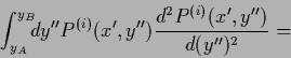
 |
(713) |
We now study density estimation problems
numerically.
In particular, we want
to check the influence of the nonlinear normalization constraint.
Furthermore, we want to compare models
with Gaussian prior factors for ![]() with models with Gaussian prior factors for
with models with Gaussian prior factors for ![]() .
.
The following numerical calculations
have been performed on a mesh
of dimension 10![]() 15, i.e.,
15, i.e., ![]() and
and ![]() ,
with periodic boundary conditions on
,
with periodic boundary conditions on ![]() and sometimes also in
and sometimes also in ![]() .
A variety of different iteration and initialization methods
have been used.
.
A variety of different iteration and initialization methods
have been used.
Figs. 14 - 17 summarize results for density estimation problems with only two data points, where differences in the effects of varying smoothness priors are particularly easy to see. A density estimation with more data points can be found in Fig. 21.
For Fig. 14
a Laplacian smoothness prior on ![]() has been implemented.
The solution has been obtained
by iterating with the negative Hessian,
as long as positive definite.
Otherwise the gradient algorithm has been used.
One iteration step means one iteration according to Eq. (617)
with the optimal
has been implemented.
The solution has been obtained
by iterating with the negative Hessian,
as long as positive definite.
Otherwise the gradient algorithm has been used.
One iteration step means one iteration according to Eq. (617)
with the optimal ![]() .
Thus, each iteration step includes the optimization of
.
Thus, each iteration step includes the optimization of ![]() by a line search algorithm.
(For the figures the Mathematica function FindMinimum
has been used to optimize
by a line search algorithm.
(For the figures the Mathematica function FindMinimum
has been used to optimize ![]() .)
.)
As initial guess in Fig. 14
the kernel estimate
![]() =
=
![]() has been employed,
with
has been employed,
with
![]() defined in Eq. (698) and
defined in Eq. (698) and
![]() =
=
![]() with squared mass
with squared mass ![]() =
= ![]() .
The fast drop-off
of the energy
.
The fast drop-off
of the energy ![]() within the first two iterations
shows the quality of this initial guess.
Indeed, this fast convergence seems to indicate that the problem
is nearly linear,
meaning that the influence of the
only nonlinear term in the stationarity equation,
the normalization constraint,
is not too strong.
Notice also,
that the reconstructed regression shows the
typical piecewise linear approximations well known
from one-dimensional (normalization constraint free) regression problems
with Laplacian prior.
within the first two iterations
shows the quality of this initial guess.
Indeed, this fast convergence seems to indicate that the problem
is nearly linear,
meaning that the influence of the
only nonlinear term in the stationarity equation,
the normalization constraint,
is not too strong.
Notice also,
that the reconstructed regression shows the
typical piecewise linear approximations well known
from one-dimensional (normalization constraint free) regression problems
with Laplacian prior.
Fig. 15 shows a density estimation
similar to Fig. 14,
but for a Gaussian prior factor in ![]() and thus also with different
and thus also with different ![]() ,
different initialization,
and slightly different iteration procedure.
For Fig. 15
also a kernel estimate
,
different initialization,
and slightly different iteration procedure.
For Fig. 15
also a kernel estimate
![]() =
=
![]() has been used as initial guess, again
with
has been used as initial guess, again
with
![]() as defined in Eq. (698) and
as defined in Eq. (698) and
![]() =
=
![]() but with squared mass
but with squared mass ![]() =
= ![]() .
The solution has been obtained by
prior relaxation
.
The solution has been obtained by
prior relaxation
![]() =
=
![]() including a mass term with
including a mass term with ![]() = 1.0
to get for a Laplacian
= 1.0
to get for a Laplacian ![]() =
= ![]() and periodic boundary conditions
an invertible
and periodic boundary conditions
an invertible ![]() .
This iteration scheme
does not require to calculate the Hessian
.
This iteration scheme
does not require to calculate the Hessian ![]() at each iteration step.
Again the quality of the initial guess (and the iteration scheme)
is indicated by the fast drop-off
of the energy
at each iteration step.
Again the quality of the initial guess (and the iteration scheme)
is indicated by the fast drop-off
of the energy ![]() during the first iteration.
during the first iteration.
Because the range of ![]() -values, being between zero and one,
is smaller than that of
-values, being between zero and one,
is smaller than that of ![]() -values, being between minus infinity and zero,
a larger Laplacian smoothness factor
-values, being between minus infinity and zero,
a larger Laplacian smoothness factor ![]() is needed for Fig. 15
to get similar results than for Fig. 14.
In particular, such
is needed for Fig. 15
to get similar results than for Fig. 14.
In particular, such ![]() values have been chosen
for the two figures
that the maximal values
of the the two reconstructed probability densities
values have been chosen
for the two figures
that the maximal values
of the the two reconstructed probability densities ![]() turns out to be nearly equal.
turns out to be nearly equal.
Because the logarithm particularly expands the distances
between small probabilities
one would expect
a Gaussian prior for ![]() to be
especially effective for small probabilities.
Comparing Fig. 14 and Fig. 15
this effect can indeed be seen.
The deep valleys appearing in the
to be
especially effective for small probabilities.
Comparing Fig. 14 and Fig. 15
this effect can indeed be seen.
The deep valleys appearing in the ![]() -landscape
of Fig. 15
show that small values of
-landscape
of Fig. 15
show that small values of ![]() are not smoothed out
as effectively as in Fig. 14.
Notice, that therefore
also the variance of the solution
are not smoothed out
as effectively as in Fig. 14.
Notice, that therefore
also the variance of the solution ![]() is much smaller for a Gaussian prior in
is much smaller for a Gaussian prior in ![]() at those
at those ![]() which are in the training set.
which are in the training set.
Fig. 16 resumes results
for a model similar to that presented in
Fig. 14, but with a
![]() -prior replacing the
Laplacian
-prior replacing the
Laplacian ![]() -prior.
As all quadratic functions have zero third derivative
such a prior favors, applied to
-prior.
As all quadratic functions have zero third derivative
such a prior favors, applied to ![]() ,
quadratic log-likelihoods,
corresponding to Gaussian probabilities
,
quadratic log-likelihoods,
corresponding to Gaussian probabilities ![]() .
Indeed,
this is indicated by the striking difference
between the regression functions
in Fig. 16 and
in Fig. 14:
The
.
Indeed,
this is indicated by the striking difference
between the regression functions
in Fig. 16 and
in Fig. 14:
The ![]() -prior produces a much rounder
regression function,
especially at the
-prior produces a much rounder
regression function,
especially at the ![]() values which appear in the data.
Note however,
that in contrast to a pure Gaussian regression problem,
in density estimation an additional
non-quadratic normalization constraint is present.
values which appear in the data.
Note however,
that in contrast to a pure Gaussian regression problem,
in density estimation an additional
non-quadratic normalization constraint is present.
In Fig. 17
a similar prior has been applied,
but this time being Gaussian in ![]() instead of
instead of ![]() .
In contrast to a
.
In contrast to a ![]() -prior for
-prior for ![]() ,
a
,
a ![]() -prior for
-prior for ![]() implements a tendency to quadratic
implements a tendency to quadratic ![]() .
Similarly to the difference between
Fig. 14 and Fig. 16,
the regression function in Fig. 17
is also rounder than that in Fig. 15.
Furthermore,
smoothing in Fig. 17
is also less effective for smaller probabilities
than it is in Fig. 16.
That is the same result we have found
comparing the two priors for
.
Similarly to the difference between
Fig. 14 and Fig. 16,
the regression function in Fig. 17
is also rounder than that in Fig. 15.
Furthermore,
smoothing in Fig. 17
is also less effective for smaller probabilities
than it is in Fig. 16.
That is the same result we have found
comparing the two priors for ![]() shown in Fig. 15 and Fig. 14.
This leads to deeper valleys in the
shown in Fig. 15 and Fig. 14.
This leads to deeper valleys in the ![]() -landscape
and to a smaller variance
especially at
-landscape
and to a smaller variance
especially at ![]() which appear in the training data.
which appear in the training data.
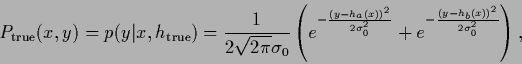
Fig. 21 depicts the results of a density estimation
based on more than two data points.
In particular, fifty training data have been obtained
by sampling with uniform ![]() from the ``true'' density
from the ``true'' density
Fig. 21 shows
the maximum posterior solution ![]() and its logarithm,
the energy
and its logarithm,
the energy ![]() during iteration,
the regression function
during iteration,
the regression function
| (715) |
 |
(716) |
| (717) |
 |
(718) |
The maximum posterior solution
of Fig. 21
has been calculated
by minimizing ![]() using massive prior iteration with
using massive prior iteration with
![]() =
=
![]() , a squared mass
, a squared mass ![]() =
= ![]() ,
and a (conditionally) normalized, constant
,
and a (conditionally) normalized, constant ![]() as initial guess.
Convergence has been fast,
the regression function is similar to the true one
(see Fig. 19).
as initial guess.
Convergence has been fast,
the regression function is similar to the true one
(see Fig. 19).
Fig. 22 compares some iteration procedures and initialization methods Clearly, all methods do what they should do, they decrease the energy functional. Iterating with the negative Hessian yields the fastest convergence. Massive prior iteration is nearly as fast, even for uniform initialization, and does not require calculation of the Hessian at each iteration. Finally, the slowest iteration method, but the easiest to implement, is the gradient algorithm.
Looking at Fig. 22
one can distinguish data-oriented from prior-oriented initializations.
We understand
data-oriented initial guesses to be those for which the
training error is smaller at the beginning of the iteration
than for the final solution and
prior-oriented initial guesses to be those for which the opposite is true.
For good initial guesses the difference is small.
Clearly, the uniform initializations is prior-oriented,
while an empirical log-density
![]() and the shown kernel initializations are data-oriented.
and the shown kernel initializations are data-oriented.
The case where the test error grows while the energy is decreasing indicates a misspecified prior and is typical for overfitting. For example, in the fifth row of Fig. 22 the test error (and in this case also the average training error) grows again after having reached a minimum while the energy is steadily decreasing.