Normalization by parameterization: Error functional

Next: The Hessians , Up: Gaussian prior factor for Previous: Lagrange multipliers: Error functional Contents

Normalization by parameterization: Error functional

Referring to the discussion in Section 2.3 we show that Eq. (141) can alternatively be obtained by ensuring normalization, instead of using Lagrange multipliers, explicitly by the parameterization

$\begin{displaymath} L(x,y) = g(x,y) - \ln \int \!dy^\prime \, e^{g(x,y^\prime )}, \quad L = g - \ln Z_X , \end{displaymath}$

(146)

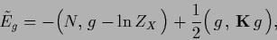
and considering the functional

$\begin{displaymath} E_{g} = -\Big(N , \, g -\ln Z_X\, \Big) +\frac{1}{2}\Big( \,g -\ln Z_X \,, \,{{\bf K}}\,(g -\ln Z_X)\,\Big) . \end{displaymath}$

(147)

The stationary equation for

obtained by setting the functional derivative $\delta E_{g}/\delta g$ to zero yields again Eq. (141). We check this, using

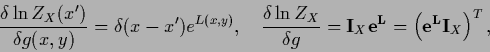$\begin{displaymath} \frac{\delta \ln Z_X (x^\prime)}{\delta g(x,y)} = \delta (x-... ...f I}_X {\bf e^L} = \left( {\bf e^L} {\bf I}_X \right)^T , \end{displaymath}$

(148)

and

$\begin{displaymath} \frac{\delta L (x^\prime,y^\prime)}{\delta g(x,y)} = \delta ... ...d \frac{\delta L}{\delta g} = {\bf I} - {\bf I}_X {\bf e^L} , \end{displaymath}$

(149)

where $\frac{\delta L}{\delta g}$ denotes a matrix, and the superscript ${}^T$ the transpose of a matrix. We also note that despite ${\bf I}_X = {\bf I}_X^T$

$\begin{displaymath} {\bf I}_X {\bf e^L} \ne {\bf e^L} {\bf I}_X = ({\bf I}_X {\bf e^L})^T , \end{displaymath}$

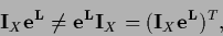(150)

is not symmetric because ${\bf e^L}$ depends on

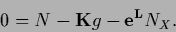
and does not commute with the non-diagonal ${\bf I}_X$ . Hence, we obtain the stationarity equation of functional

written in terms of

again Eq. (141)

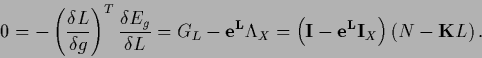$\begin{displaymath} 0 = -\left( \frac{\delta L}{\delta g} \right)^T \frac{\de... ...} - {\bf e^L} {\bf I}_X \right) \left(N- {{\bf K}} L \right) . \end{displaymath}$

(151)

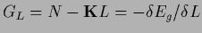Here $G_L = N - {{\bf K}} L = -\delta E_g/\delta L$ is the

-gradient of

. Referring to the discussion following Eq. (141) we note, however, that solving for

instead for

no unnormalized solutions fulfilling $N={{\bf K}}L$ are possible.

In case $\ln Z_X$ is in the zero space of ${{\bf K}}$ the functional corresponds to a Gaussian prior in alone. Alternatively, we may also directly consider a Gaussian prior in

$\begin{displaymath} \tilde E_{g} = -\Big(N , \, g -\ln Z_X\, \Big) +\frac{1}{2}\Big( \,g\,, \,{{\bf K}}\,g\,\Big) , \end{displaymath}$

(152)

with stationarity equation

$\begin{displaymath} 0= N -{\bf K} g - {\bf e^L}N_X . \end{displaymath}$

(153)

Notice, that expressing the density estimation problem in terms of

, nonlocal normalization terms have not disappeared but are part of the likelihood term. As it is typical for density estimation problems, the solution

can be calculated in

-data space, i.e., in the space defined by the

of the training data. This still allows to use a Gaussian prior structure with respect to the

-dependency which is especially useful for classification problems [236].

Next: The Hessians , Up: Gaussian prior factor for Previous: Lagrange multipliers: Error functional Contents

Joerg_Lemm 2001-01-21