Inverse and direct problem of the Heat equation in 1D

We examine a heat problem in 1D. Assume that a rod with given temperature distribution u_0(x) is cooled to temperature 0 on the exteriors at 0 and pi. Assume that u(x,t) for the Temperature at point x and time t satisfies the Heat equation

with boundary conditions

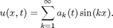
Compute the coefficients of the sine series

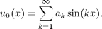
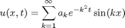
Then the analytical solution to the heat problem is given by

Proof: Denote by a_k(t) the coefficients of the sine series at each point t in time

Inserting into the equation yields

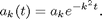
with the solution

In the following, we demonstrate this solution and ask whether we can also solve the backward Heat equation: Given the value of u(x,T) for some T>0, can we compute u(x,0)=u_0(x)?

Initialization
Compute Sine coefficients
Compute solution to the forward problem
Inverse Problem
Setup
Solve the inverse problem
What's wrong?
So what happened?
What can we do?

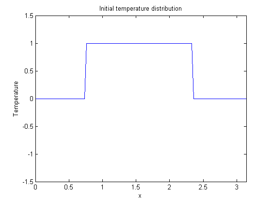
Initialization

% We solve the forward problem with initial data given at 0.
% We choose N discretization steps in the x direction on [0,pi], n steps in
% the t direction on [0,T].
N=128;
n=128;
T=0.1;
% Set up the initial function u0. We choose the characteristic
% function of pi/4..3 pi/4.
u0=zeros(N,1);
u0(N/4:3*N/4)=1;
% Since core matlab has no built-in sine transform, we replicate the
% vector of initial values with reversed sign and take the Fourier
% transform, this is the same as taking the sine transform which is
% then in the imaginary part. This is
% actually a joke - providing a dst is a one-liner when you have fft.
% And even worse: Matlab uses fftw to compute the fft, which *does* have a
% sine and cosine transform, but charges extra for its definitions in the PDE
% and imaging toolboxes. Weird.

u0(2*N:-1:N+2)=-u0(2:N);
x=(0:2*N-1)/N*pi;
% Display the initial temperature distribution we are starting with.
subplot(1,1,1);
plot(x,u0);
xlabel('x');
ylabel('Temperature');
axis([0 pi -1.5 1.5]);
title('Initial temperature distribution');

Compute Sine coefficients

Next, we compute the sine coefficients of u0. As mentioned above, core matlab has no sine transform, so we apply the fft to u0 on [-pi,pi] continued as an odd function.

% Set up a matrix in which all columns are the same as u0.
A=u0*ones(1,n);
% Compute the sine (or Fourier-) coefficients in each column.
A=fft(A);

Compute solution to the forward problem

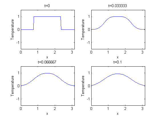
Now that we have the sine coefficients a_k of u0, we can solve the initial value problem by computing u(x,t) using the series above. Since explicit summation would be slow, we apply the fast inverse sine transform. So all we do is multiply the sine coefficients computed above with the degradation factors in the sum and take the inverse sine transform.

Notice that we multiply the sine coefficients with very small numbers. Even for moderate t, exp(-k^2*t) is numerically zero for most k. Also note that it is very hard to see any difference between the last images. While the diffusion process is visible at the beginning, it slows down fast.

% Multiply Fourier coefficient a_k(t) = a_k exp(-k^2 t).
t=(0:n-1)/(n-1)*T;
k=[0:N-1 -N:-1];
k2=k.*k;
W=k2'*t;
W=exp(-W);
A=A.*W;
% Take the inverse sine (or Fourier-) transform.
u=real(ifft(A));
% Ok - that's it, u now has the solution.
% Display the result for various times.
subplot(2,2,1);
plot(x,u(:,1));
title('t=0');
axis([0 pi -1.5 1.5]);
xlabel('x');
ylabel('Temperature');
subplot(2,2,2);
plot(x,u(:,round(n/3)));
title(['t=' num2str(T/3)]);
xlabel('x');
ylabel('Temperature');
axis([0 pi -1.5 1.5]);
subplot(2,2,3);
plot(x,u(:,round(2*n/3)));
title(['t=' num2str(2*T/3)]);
xlabel('x');
ylabel('Temperature');
axis([0 pi -1.5 1.5]);
subplot(2,2,4);
plot(x,u(:,round(n)));
title(['t=' num2str(T)]);
axis([0 pi -1.5 1.5]);
xlabel('x');
ylabel('Temperature');

Inverse Problem

So solving the initial value problem with data given at time t=0 works. We now turn to the backward (inverse) problem: Assume that we measure temperature u(x,T) at time t=T>0. Can we recover u0 from this measurement?

The idea is simple: The sine coefficients of u(x,T) are simply those of u0 multiplied by exp(-k^2 T), so given u(x,T) we take its sine transform, multiply by exp(k^2 T) - theses are the sine coefficients of u0. We arrive at u0 by taking the inverse sine transform.

Setup

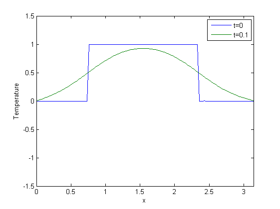
First, extract data and u0 from u and display both.

daten=real(u(:,n));
truesolution=real(u(:,1));
subplot(1,1,1);
plot(x,truesolution,x,daten);
axis([0 pi -1.5 1.5]);
xlabel('x');
ylabel('Temperature');
legend('t=0',['t=' num2str(T)]);
%xcolview(u);

Solve the inverse problem

Take the sine transform an multiply by exp(k*k*T). Take the inverse transform and plot.

fdaten=fft(daten);
E=exp(k2'*T);
fguess=fdaten.*E;
guess=real(ifft(fguess));
subplot(1,1,1);
plot(guess);
axis([0 pi -1.5 1.5]);
xlabel('x');
ylabel('Temperature');

What's wrong?

Definitely, that didn't work - we get no plot at all. The reason is that E is a matrix of very large numbers - easily exceeding the max float, so that E contains mostly Infinite numbers. Let's count the number of Infs and the number of elements in E with size bigger than 1E8.

sum(sum(E==Inf))
sum(sum(E>1E8))

ans =

    87


ans =

   229

So what happened?

The sine coefficients of u were multiplied by very small numbers, many of them actually numerically zero. Trying to recover them is impossible - they are gone for good.

While one might argue that higher precision arithmetic would have solved this problem, this is irrelevant in practice. Assume that u(x,T) is not given a priori, but as a measurement. Multiplying its sine coefficients by a number and taking the inverse transform means multiplying the measurement error by that number, and this quickly becomes unacceptable.

What can we do?

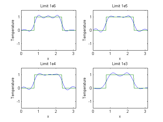
Since most of the sine coefficients are gone anyway, we just should not try to recover them. In the multiplication with exp(-k^2 T) above, we must restrict ourselves to "small" values. In the following, we choose some limits and show the corresponding results, always comparing with the true solution.

%plot for limit 1e6
subplot(2,2,1);
M=find(E>1e6);
E(M)=0;
fguess=fdaten.*E;
guess=real(ifft(fguess));
plot(x,guess,x,truesolution);
axis([0 pi -1.5 1.5]);
xlabel('x');
ylabel('Temperature');
title('Limit 1e6');
%plot for limit 1e5
subplot(2,2,2);
M=find(E>1e5);
E(M)=0;
fguess=fdaten.*E;
guess=real(ifft(fguess));
plot(x,guess,x,truesolution);
axis([0 pi -1.5 1.5]);
xlabel('x');
ylabel('Temperature');
title('Limit 1e5');
%plot for limit 1e4
subplot(2,2,3);
M=find(E>1e4);
E(M)=0;
fguess=fdaten.*E;
guess=real(ifft(fguess));
plot(x,guess,x,truesolution);
axis([0 pi -1.5 1.5]);
xlabel('x');
ylabel('Temperature');
title('Limit 1e4');
%plot for limit 1e3
subplot(2,2,4);
M=find(E>1e3);
E(M)=0;
fguess=fdaten.*E;
guess=real(ifft(fguess));
plot(x,guess,x,truesolution);
axis([0 pi -1.5 1.5]);
xlabel('x');
ylabel('Temperature');
title('Limit 1e3');